THE TECHNION PHILADELPHIA FLIGHT CONTROL LABORATORY ANNO 1971
A History
This is the story of the Flight Control Laboratory at the Faculty of Aerospace Engineering of the Technion. It is a tribute to the late Professor Shmuel Merhav, who started the laboratory in 1971 from scratch, and who’s vision let to developments that were their time far ahead. Today the Laboratory is a thriving exciting place, on the forefront of autonomous navigation, perception, and cooperative autonomous systems. Many techniques and systems that are commonly used today are rooted in a long evolutionary process that took place all through the 50 years of existence of the laboratory. Today’s students and researchers take existing tools and software packages like Matlab, Simulink, LabView, Mathematica, Solidworks, 3-D printing, etc. for granted. However, none of these tools existed and inventiveness, creativity and vision were required to carry out flight control research under stringent budgetary restrictions.
How it started
In September 1971 Professor Shmuel Merhav, shown in Figure 1, left RAFAEL, the Israeli Armament Development Authority, to start a new Flight Control Laboratory at the Faculty of Aerospace Engineering. For this purpose, the Faculty dedicated a dark and dusty space, adjacent to the transonic wind tunnel, located at the Aeronautical Research Center. The place was fenced off from the rest of the complex by a two-meter-high corrugated plastic fence. Apart from two work benches, a table, and some chairs the place was empty. The laboratory equipment consisted of one oscilloscope, a few soldering irons, and a small mechanical work bench. The laboratory staff consisted of the chief electronic engineer, Yeheskel Ben-Arie, and two technicians Elhanan Rabinovitch and Benni Cooper.
Professor Itzhack Bar-Itzhack, shown in Figure 1 right, joined the Faculty at the same time, and his research interests were in Inertial Guidance and Navigation Systems. Two PhD students joint Professor Merhav in his efforts to build the laboratory. The focus of interest was research on pilot-vehicle systems, flight control and aerospace guidance and navigation.

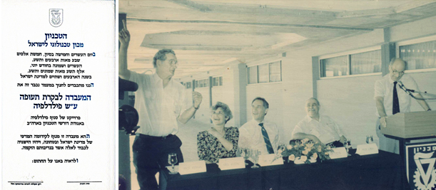
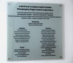
Figure 2: PFCL Dedication Plaque
The laboratory thanks its name to the Philadelphia Chapter of the Technion Society, whose members adopted the Laboratory 18 years later, in the year 1989. The Chapter contributed to a large part of the computational equipment and electronics in the laboratory, that has been imperative in a wide range of research activities for years to come. Figure 2 left, shows the foundation plaque.
We go again back to the year 1971. The laboratory’s first breakthrough was the acquisition of a used EAI analog computer, donated by the Faculty of Electrical engineering. This computer consisted of many operational amplifiers that could be wired to solve sets of differential equations in real time. Digital real-time simulation was impossible at that time and would require a fully devoted CDC Cyber computer or IBM main frame. The analog computer was essential in simulating the dynamic response of aircraft in real time. Programming of this computer took place by plugging colorful wires into a removable patch board, on which connections were made to the operational amplifiers. The only problem was that the laboratory was next to the transonic wind tunnel and each time this tunnel was operated, the noise and vibration would shake the room and the amplifiers would become unbalanced. Fortunately, Elhanan quickly learned to repair the faulty amplifiers.
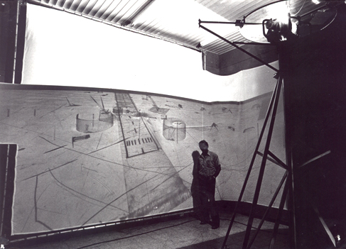
Figure 3: Shadowgraph Simulator (1973)
The first visual flight simulators
The first efforts were devoted to building a flight simulator. Computer graphics was non-existing and the images needed to be generated by optical systems and servo drive hardware. The first system was based on the ‘shadowgraph’ principle, shown in Figure 3. The design consisted of a large circular transparent Perspex disk, containing the outline of a visual scene. A bright halogen point-source lamp projected a shadowed image on a large screen, as seen from the viewpoint of the point source. The slide could move in two dimensions, driven by two servo-controlled rollers, forward and yaw. A third dimension was added by moving the light source up and down. All parts were designed and manufactured in-house as well as the power supplies, power amplifiers and electronics necessary to move the slide. The shadowgraph was not completed until 1973, where it was placed in the high bay of a new location. The picture in Figure 3 shows Professor Merhav next to the shadowgraph screen. Unfortunately, it was never used in research. The motions were too jerky and unreproducible, the motion space too limited and it lacked degrees-of freedom for effectively simulating the motions of an aircraft. However, it was sometimes used by the students as a primitive toy for executing dive-bombing on the scene, because when the hot lamp would hit the plastic models on the slide, they would start to smoke.
In the early 70th remotely piloted vehicles or RPV’s were in their infancy. It was the ambition of a few model airplane enthusiasts rather than being considered for any civil or military missions. Early on, Professor Merhav saw the potential of RPV’s and started research projects directed at the effective manual control of RPV’s. The first thought was that these RPV’s should be controlled by means of a vehicle-based camera, rather than by an operator, visually controlling it from the ground. For this we needed a simulator and we spent already too much time on the shadowgraph.
Figure 4: RPV Simulation Setup (1975)
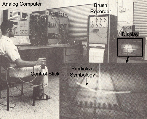
Figure 5: Predictive symbols, generated on a separate stroke-written CRT, overlaid on the scene
A 5-degrees-of-freedom RPV simulator was constructed from a discarded viewgraph projector of which the projection head was fitted with a servo motor as shown in Figure 4, left. A servo-driven transparency belt with a dotted landscape pattern was looped around the viewgraph and the moving picture was projected on a large screen on the wall thus creating forward and lateral motion. A two-axis mirror servo with a vidicon camera was mounted on a servo-controlled carriage that could move to and from the wall, enabling yaw, pitch, and vertical degrees of freedom, as seen in Figure 4, right. The simulator was built mainly from salvaged parts in less than 3 months. The vehicle motions were programmed into the analog computer, responding to the manual inputs from a control stick.
It became soon clear that landing the RPV by means of the vehicle-based camera image was extremely difficult and that image stabilization and superimposed display aids were required to successfully perform this task. Predictive symbols generated on a separate stroke-written CRT were overlaid on the scene as seen in Figure 5. Note that this setup was completely analog: the analog computer that hosted the vehicle dynamics, the control stick, the brush recorder, and the screen. Although the system was complex and the various components needed frequent and accurate calibration, the simulations were extremely revealing and helped to device methods for controlling RPV’s by remote presence. During a visit of the Apollo astronauts at the Technion, after flying the simulator they commented that the dotted landscape reminded them of the moon landing, see Figure 6. Other unforgettable visitors, flying the simulator, were the Egyptian and Israeli ministers of defence, Ali and Weizman, during the visit of President Sadat in 1979.
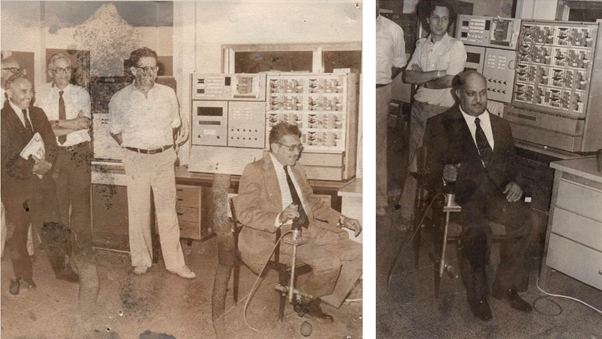
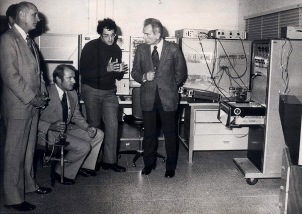
Figure 6: Visitors to the lab flying the simulator: above: Ali and Weizman, below: Apollo crew
The first building
Fortunately, in 1973 the laboratory moved to a new building. It was a one-story prefab building with two large rooms of which one had a high ceiling to accommodate the shadowgraph. A number of small rooms to the side served as offices for the staff and graduate students. The building was in the middle of nowhere, on the road to the defunct site of the planned Technion atomic reactor. It was lately taken down when the Asher Space Research Institute was built next to it. The nature was stunning, and it was a happy time in a quiet place, away from the wind tunnel. You just needed to put your hand outside the window to obtain all the leaves for an herbal tea.
We received a second EAI analog computer, also donated by the Faculty of Electrical engineering. Other pilot-vehicle related research included parameter estimation of the human response in manual tracking tasks. Modelling the human operator transfer function is vital in understanding how the operator interacts with the fight vehicle. Other subjects dealt with active control manipulators, kinaesthetic feedback and manual control with sampled-data. Two more M.Sc. students joined the laboratory and soon there were not enough colored wires available for all of us to program the analog computers.
The first digital computer
In 1974 the laboratory received its first digital computer, a Data General Nova 2. It had 32 Kbytes of memory with a word length of 16 bits. A paper tape was used to program the computer in assembly language, and it had 4 registers. A teletype was used to punch and read the tapes. It was tedious and time-consuming work and sometimes a tape would break and then you needed to start the punching all over again. The cycle time of a no-op was 2 microseconds. Being used to the Technion’s IBM 360/365 main frame computer, having our own computer in the laboratory was heaven, and we regarded it as an absolute wonder. We purchased an analog-to-digital converter that came in a large metal frame and a digital tape drive to record the dynamic response of the pilot vehicle system. Being able to record and post-process experimental data was a huge step forward from the analog recording on the brush recorder. Identification of the human operator response took place both in the frequency domain by Spectral Density Distribution methods, as well as in the time-domain, by more advanced recursive parameter estimation methods.
I remember working with a colleague recording the human response of the operator in a tracking task. After a day of recording, we sent the tape to the Taub Computer Center, where the contents would be transferred to the IBM 360/365 for off-line processing. After a few days, the results came back in de form of a stack of 50 pages of compute printout with only zeros! We did not understand what had happened and I asked my colleague if he had switched on the analog-to-digital converter. He said ‘no, did you?’
Pilot-Vehicle modelling
In that time Human Operator modelling was the focus of research of the laboratory. Two competing human operator modelling concepts existed in literature: McRuer’s ‘Cross-Over Model’ based on classical control theory, and ‘the Optimal Model for Human Response,’ from BBN Boston MA, based on linear quadratic optimal estimation and control theory. These two mainstreams were battling each other at the stage of the yearly ‘Annual Conference on Manual Control’. Both concepts were used in our lab, and Kalman filtering was a new and exciting subject. However, linear algebra packages for solving the Riccati equation were non-existing, so we wrote our own packages through endless iterations on the IBM 360/650 main frame of the Technion.
The IBM 360/365 main frame computer
The main frame was accessed by means of a huge card reader in a small room in the Aeronautical Engineering building. A few machines were available to punch the cards that would contain your program. The main frame had 4 classes: class A featured a mere 32Kbytes of memory for your program. For your ‘larger’ programs you needed to run overnight in class B of 64Kbyte and class C and D were reserved for special operations like reading magnetic tapes. The roundabout time for a program was about half a day and the output came back to you in a printout on a stack of wide-format paper. The programs were written in Fortran and the pack of cards needed 4 incomprehensible ‘Job Control Language’ cards or JCL header. From time to time the code on these cards would change for some typical IBM reason, and you would spend half a day figuring out how to get it running again. Frequently the reader got stuck or the connection with the computer center was interrupted. Sometimes your card pack fell scattering all cards on the ground. Display screens did not exist in that time and the only communication with the main frame was through a teletype.
The reason I write this is to compare it with today’s highly intuitive human interfaces and lightning-fast response times. But we regarded the IBM 360/365 as an absolute wonder and managed to put together the linear algebra package with careful planning and thinking. Plotting of graphs was hardly possible. Your output could be directed to a pen plotter at the computer center, and it would take a few days to get the results through the Technion internal post. The IBM had a dynamic simulation program called CSMP or Continuous System Modelling Program. The results came in the form of a dotted symbol graph printed on a wide belt of IBM paper sheet. Today we would cringe at the waste of paper it produced.
In these pre-Matlab/Simulink times, tools like Root Locus, classical control design tools and graphics representation were non-existing and we had to develop them ourselves. There existed a rudimentary Scientific Subroutine Package, called SSP, that included some basic matrix operations that was of some help. In 1974 Professor David Kleinman from Storrs, CT came to the Technion on a Sabbatical. He brought with him a box of punch cards he called ‘Linpack.’ It was a linear algebra package that included everything we needed. We were amazed to learn how the Riccati equations were efficiently solved. Today research students would be completely lost without Matlab or Simulink. Furthermore, the computational power of personal computers allows to view the dynamic response of systems in real time, sometimes in the form of complex 3-D graphics representations which was unheard of in that time.
The first flight control and navigation courses
Professor Merhav wrote and introduced a number of essential courses, vital in the flight control area. These courses encompassed the basic tools for the research students in the laboratory. The flagship course ‘Automatic Flight Control’ was based on the books of McRuer and Blakelock and are up till now essential parts of the curriculum. Optimal control, parameter estimation and random processes, geared towards Aerospace, became essential prerequisites for graduate students. His iconic ‘Aerospace Sensor Systems’ course was archived in book form, and communicated the present-day concepts that different sensors should not work by themselves but must be integrated in a complementary filtering system. Professor Bar-Itzhack wrote his very popular course ‘Inertial Navigation,’ which clearly explained the intricacies of gyros, coordinate transformations and inertial platforms and was highly appreciated by both undergraduate and graduate students.
The vibrating Coriolis angular rate sensor
Professor Merhav believed that signal processing and random processes were vital tools in Aerospace Control. Partly inspired by the Aerospace Sensor Course he was teaching, he became interested in finding alternatives for the classical rate gyros. He pioneered the concept of the vibrating Coriolis angular rate sensor, which is presently incorporated in any appliance or device you can think of in the form of a solid-state chip. He built a prototype, together with Elhanan Rabinowitz, consisting of two highly precise accelerometers, mounted on a vibrating arm. Through a clever analog decoding scheme, the rotational rates could be measured. However, the table on which the device was resting was not ridged enough and its flexing modes became artifacts in the measurement. To create a stable surface, a one-meter-deep hole was dug in the floor of the laboratory and filled with concrete to create a solid base for a pedestal. The setup was placed on the pedestal and Professor Merhav’s goal of measuring the Earth angular rates was realized. When we asked him how he got to these amazing results, while Professor Bar Yitzhack was more the authority on inertial systems, he jokingly answered ‘well sometimes it is good not to be bothered by too much knowledge.’
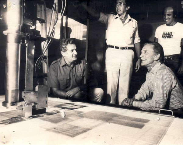
Figure 7: Four axis light table with actor Kirk Douglas
Image processing and motion detection
In the mid-70th Professor Merhav introduced image processing in Aerospace Applications in the laboratory. The chief laboratory engineer Yeheskel Ben-Arie was the driving force in this area. A Vicom Digital Image Processor was acquired. An exciting line of new research projects was spun-off. The focus was on image enhancement, motion detection and terrain-aided navigation. A high-precision four-axis light table was built. slides of aerial photographs were placed on this table, that could move in x-y direction. Figure 7 shows actor Kirk Douglas near this table during his visit at the laboratory. The camera could move up and down and a servo-controlled focusing system kept the image crisp and sharp. Since at that time all processing was analog, a very unique system was developed for electronically manipulating the image in roll and slant. This effectively added two additional degrees-of-freedom to the system without the need for physically rotation the camera. The table with its analog roll and slant system became so successful that a second larger table was built on this concept for RAFAEL.
Apart from managing the laboratory, Yeheskel Ben-Arie was involved in research on computer vision and shape recognition, which was also the subject of his PhD thesis. After finishing his thesis, Yeheskel moved to the US where he pursued a very successful carrier in this area. One interesting research project involved aiding the gyro compassing of satellites, based on motion detection of a down-looking camera. Other research topics dealt with terrain-aided navigation. Soon the research shifted from correlation techniques to the recognition of shapes and forms.
The image processing activity drastically increased the number of graduate students and programmers in the laboratory. A Data General Eclipse computer was acquired, to satisfy the computational demands of the students. The computer had 4 slots of 32Kbyte of memory, the word length was still 16 bytes and it came with hard drive of 96 Mbyte of memory which had the size of a large Maytag washing machine. It had the RDOS operating system which allowed the computer to be programmed from a terminal instead of having to use paper tapes. It even had a Fortran compiler and two users could work on the computer at the same time: one in the ‘foreground’ and one in the ‘background.’ However, the system was badly protected, so that if one user crashed the computer, the other one lost her/his data as well. The hard drive used a heavy pack of stacked disks, and several of these disk packs were acquired to satisfy the needs for space for the recorded images used in the image processing research. Dust in the air from the nearby building site of the Canada building, frequently caused these disks to crash. The Eclipse has lately found his final resting place in the Madatech Israel National Museum of Science, Technology and Space in Haifa.
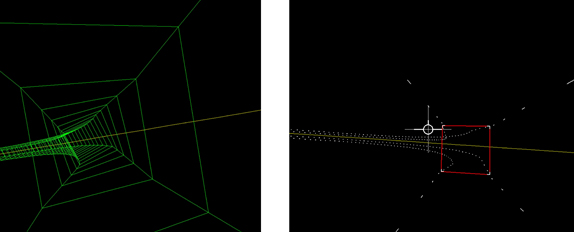
Figure 8: Stroke-written images of the ‘Tunnel in the Sky’ display
The first stroke-written computer graphics
The terminals were basically line editors and could not display graphics. However, real-time graphics was needed in the pilot-vehicle research. The graphic images were displayed as green lines on a large and expensive HP oscilloscope with electrostatic deflection. The image was generated by an HP fast plotter in the form of a stroke-written image, driven by the Eclipse Computer. Since the Eclipse did not have floating-point hardware, it was not fast enough to program the image in Fortran, so tedious assembly programming was required. Vehicle motions were still generated by the analog computer and imparted to the Eclipse through the analog-to-digital converter. This was the first time that visual flight could be simulated by electronic means only, without the need for mechanical servo drives. Figure 8 shows images of the ‘Tunnel in the Sky’ research, in which the 3-D winding and descending flight path that needed to be followed was presented to the pilot as a tunnel in the sky. The image on the right of Figure 8 shows a predictor symbol with tunnel cross-section, at an appropriate lead distance ahead. The predictor symbol was found to be imperative in effortlessly following the tunnel. Note that this picture was actually stroke written monochrome green and has been reproduced here in color for illustration.
This spun-off several other projects, one of which dealt with reducing the workload in agricultural flight, in cooperation with Chim-Nir Aviation, Herzliya. In this research a path predictor symbol was overlayed on the visual field. Although the CHim-Nir pilots very much liked the concept, they said that they would actually be more pleased by having an air conditioning system installed in their Rockwell SR-2 crop duster. A three-beam color video projector was used to project the agricultural scene on a large screen in front of the pilot. This projector was very large and heavy in comparison to presently used projectors and a dedicated support system had to be built. No scan converters existed to translate the stroke-written image on the CRT to the projected video image, so we simply did this by placing a camera in front of the CRT.
The late 70th was also the time mechanical cockpit instrumentation was being replaced by digitally generated images. The Head-Up display was seen as a promising concept in which digitally generated images were overlayed on the outside visual field. This was important in situations in which the pilot needed to keep her/his full attention on the outside visual field. An interesting project dealt with the landing of helicopters on moving ship deck. A visual simulation was carried out in which inertially stable visual references and predictive information was displayed to aid the pilot in safely touching down on the moving ship deck.
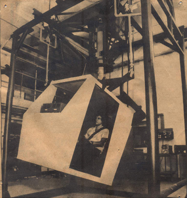
Figure 9: Three-degrees-of-freedom motion simulator
Moving base simulators
In the early 80th the laboratory moved to its present location in the newly inaugurated Lady Davis building. It was spacious and new and had two high-bays. One of the rooms was dedicated to a moving base simulator. It had three-degrees-of-freedom and was designed and build in-house. A cabin was suspended from above by three servo-driven rods as shown in.Figure 9. By operating these rods collectively, the cabin would heave, and differentially it would pitch and roll. The static weight was supported by a cantilever beam with air spring. Professor Merhav named this setup the ‘Yoyo Simulator.’
Professor Merhav decided to build this simulator for research on suppression of biodynamic interference. This interference appears in buffeting flight in which the aircraft vibrations are transferred through the body and arm of the pilot to the control stick. These unwanted control inputs might become amplificated in the control loop leading to catastrophic conditions. Professor Merhav intended to suppress the biodynamic interference by means of the adaptive noise cancellation method developed by B. Widrow. In this method the vibrations measured by a sensor outside the vibration environment of the stick are passed through an adaptive filtering algorithm, thus creating a signal used to remove the unwanted control inputs.
The simulator would serve as the vibration base. The problem with this simulator was an inherent lack of stiffness, causing the structure to resonate heavily in certain frequencies. We decided to stiffen the simulator by attaching it to the wall by means of several metal rods. However, the vibrations were so strong that the rods broke free from the wall. We realized that shortcuts were not possible here and the structure was eventually heavily anchored to a steel support beam. In spite of this problematic simulator concept, the method was highly successful and led to several research contracts with the NASA Ames Research Center in California.
In 1985, spun-off by the success of the research on suppression of biodynamic interference, Professor Merhav decided to develop a better motion platform. This time it was based on a 6-degrees-of-freedom Stewart Platform. Mr. Steve Meadow from California donated $100,000 for this project. In contrast to the previous three-degree-of freedom simulator, the Steward Platform system is statically defined and virtually free of resonant modes.
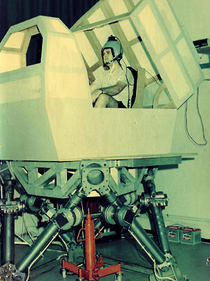
Figure 10: 6-degrees-of-freedom Stewart Platform with wooden cabin
Several actuator options were considered. Hydraulic actuators would ensure very smooth motions and a high bandwidth response, but were too costly. They would also need to be submitted to stringent safety protocols for use with human subjects. The alternative was an electro-mechanical system with linear actuators that were not commercially available at that time. A unique system was designed and build in-house. Even the high-current power supplies and amplifiers were built in-house since off-the-shelf products were either unavailable or too expensive. Each one of the six linear actuators was driven by two inland torque motors. The original design included a rack-and-pinion to transform the rotational motion into a linear one. This arrangement proved far too noisy and was replaced by a steel cable looped around the spindle of the torque motors. It was mechanically equivalent to the rack-and-pinion, but yielded a markedly smoother motion. A wooden cockpit was placed on the platform as shown in Figure 10.
The full range of the six degrees of freedom was never fully utilized. Most of the projects involved biodynamic interference, where the platform was used as a vibration base, exciting the platform only in fast and small-amplitude heave or pitch motions. One interesting project included the effect of biodynamic interference on the visual accuracy in helmet-mounted displays. The idea was to use the adaptive filtering technique for stabilizing the image. This project was done in cooperation with the NASA Ames Research Center under a MOU agreement. An earthquake in the San Francisco Bay area rendered the Ames simulators temporarily inoperative. Therefore, the US pilots came to the Technion to perform the task with our simulator.
The shortcomings of the cable-driven system became soon apparent. The small and fast motions of the platform caused the steel cables to wear out fast and they would break after one day of experiments. Only one mechanical workshop technician was intricately familiar with the complex design and he would work most of the night to replace the broken cable, so that the US pilots could continue the experiment the next morning.
The vulnerability of the cables to wear-and-tear has been a problem until today. In order to alleviate this problem a ‘seventh-leg’ support system was added, consisting of a pneumatic air cylinder connected to a pressure tank. The pressure in the cylinder would be adjusted such, that the static weight of the platform would be cancelled out and the cabin would be ‘floating.’ This arrangement not only drastically improved the life time of the cables, but also its smoothness of motion.
At present, the platform no longer serves as a flight simulator. It will be used to study the behavior of people standing on a moving platform like in public transport. It is still a unique system where the original analog electronic control system is retro-fitted with an up-to-date digital system based on a National Instruments Compact RIO. Since the system is now computer-controlled, many essential safeties featured could be incorporated. This system is well documented as well as the complex method for replacing the broken cables. At the moment we are experimenting with Kevlar cables with promising results. We hope that this unique system, build and designed in the 80th will still have a useful life time.
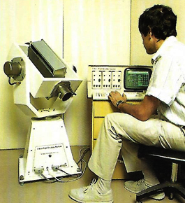
Figure 11: Elhanan Rabinovitz working on the 3-axis flight table
High-accuracy 3-axis flight table
Professor Bar Itzhack wrote the specifications for a high-precision 3-axis flight table that was designed and build by Moked Engineering, Jerusalem. The table had highly accurate shaft encoders and could rotate with the accuracy of degrees-per-hour. It was extensively used as a platform for research on strap-down systems using Kalman Filtering. In other research it serves as the motion base for a seeker head. Today it is still used as a testbed for hardware-in-the-loop simulations of UAV guidance and navigation equipment. The basic analog servo drive system is still operating flawlessly, while being controlled by Matlab digital simulation software.
In the area of navigation, efforts were directed to find alternatives for costly, high-precision inertial sensors like the vertical gyro and rate gyros. The efforts were in-line with the courses that both Professor Merhav as well as Professor Bar Yitzhak were teaching on aerospace sensor systems and inertial navigation. The idea was to fuse the output of a number of low-cost different sensors in a complementary estimation scheme in order to replace the costly gyroscopes. Kalman filtering schemes were used extensively and the laboratory became a ‘center of knowledge’ advising both Elbit and the Ministry of Defense in various projects. The Moked 3-axis flight table was an invaluable piece of equipment in these efforts. In a later stage a Trimble GPS system was purchased. It came in the form of a large yellow box, and a large GPS antenna disk needed to be placed on the roof of the building. At that time, high accuracy GPS was only selectively available (SA), and one of Professor Bar Yitzhak’s projects studied algorithms to circumvent the selected availability.
Advanced real-world image generation
In the 90th the laboratory purchased its first image generation computer from Silicon Graphics. This company was a leader in real-time computer-generated imaging. It was an expensive purchase but jump-started a series of visual flight control experiments that were not possible earlier. Today, the advent of computer gaming has resulted in high-performance low-cost graphics cards that have put Silicon Graphics out of business. Their unique graphics programming language GL is still widely used in open form. Today, any off-the-shelf laptop computer has built-in graphics capabilities that were unheard off at that time.
The ability to render real-world images, opened possibilities that were not earlier possible with stroke-written displays. One research projects dealt with dichoptic vision when using a monocle Helmet-Mounted Display. The outside real-world view was projected on a screen, while the flight information was displayed on the monocle. This required the pilot to switch her/his attention between the two images under these unnatural conditions.
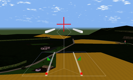
Figure 12: Scene-linked visual augmentation in a precision hover task
A different project studied the control-oriented visual information in low-altitude visual flight. It was investigated how well a subject was able to derive the straight or curved predicted vehicle path from the visual streamer pattern, while flying over a textured surface. Another project dealt with the development of Helicopter Integrated Pictorial Displays for flying complex re-routable approach trajectories. Head-Up and Head Mounted Displays made it possible to incorporate visual augmentation as part of the outside visual field. An example of this scene-linked information for a precision hover task is shown in Figure 12.
A totally different project dealt with a novel method for workload assessment in visual flight by means of Peripheral Arterial Tone (PET) measurement. The PET method was developed for studying sleeping disorders in which the subject is at rest. A flight over an agricultural scene with various levels of difficulty was chosen as the test case. The PET is measured by a pneumo-optical probe placed on a finger. However, in flight the pilot moves her/his hands resulting in artifacts in the measurements that needed to be removed in post-processing.
Hovering Vehicles
In the year 2000 we decided to explore the area of indoors manual controlled hovering vehicles. The development was intended for the exploration of structures unfit for human access. Today’s multi-rotor drones did not exist yet. Although rotor blades were the obvious choice for this development, we wanted to use the concept of the cyclorotor, which seemed to us far more challenging. It uses a horizontal-axis cyclorotor, to provide lift, propulsion and control. The rectangular blades of the cyclorotor would rotate along the circumference of a cylinder as shown in Figure 13 bottom left. Through an eccentric link, the pitch of the blade could be varied collectively or cyclically, thus modifying the magnitude and direction of the lift vector.
Four cyclorotors were placed in a star-like configuration as shown in Figure 13 top right. By controlling the lift vector of each rotor, three independent forces and three independent moments could be generated as depicted by the arrows and circles in Figure 13 top left. This would allow the vehicle to maneuver omnidirectionally, while keeping it perfectly level thus eliminating the need for a gyrostabilized camera.
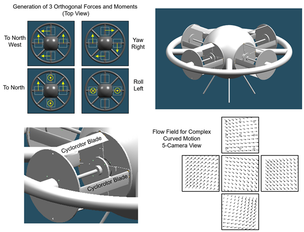
Figure 13: The Cyclorotor hovering vehicle
In order to stabilize and control the vehicle we intended to use the optical flow from vehicle-mounted cameras. A feasibility study was carried out using the 3-axis flight table to generate motion patterns. Figure Figure 13 bottom right, shows the 5-camera flow field for complex motion. A correlation technique was used to sample the flow field at various locations in the image. A complementary filtering scheme was developed to blend the flow field measurements with inertial sensor data. Today, using the flow field for stabilization is an almost standard feature of commercial drones.
One cyclorotor was designed and built and tested in the laboratory. Although the lift vector could be adequately controlled in magnitude and direction, the shortcomings of this concept became soon apparent. To create sufficient lift, the rotational speed needed to be extremely high, causing high bending moments on the rotor blades. The bending of these blades could be visually noticed, and all experiments were conducted behind a plexiglass safety shield. It is hard to compete with the effectiveness of conventional rotor blades in which the stresses are along the axis of the blade. This is apparent in today’s exclusive use of fixed-pitch RPM controlled multi copters.
Although a 50 cm diameter prototype was fully designed with sensors, actuators, and control system electronics, it was never built due to the high cost of the components. It took several more years for the first quad and multi-rotor crafts to emerge on the market. Obviously, a fixed-pitch speed-controlled rotor blade is the best choice for small multi-rotor vehicles. But commercially available RPM controlled motors for this solution and its integrated electronics were only available many years later. Likewise, high resolution miniature cameras and low-cost solid state inertial sensors, magnetometers and GPS receivers, were something we could only dream of. Of-the-shelve low-cost solutions for control and navigation of miniature drones are presently available with gimbal-mounted stabilized cameras, making it unnecessary to keep the vehicle perfectly level. Today, a vast market of low-cost, highly augmented automated drones with gyro-stabilized cameras are commonly available consumer products, and can be flown by any lightly trained person.
Hovering vehicle simulator
In order to create realistic motion patterns of a hovering vehicle, it was necessary to mount the cameras and inertial sensors on a platform that could move through the room in six degrees of freedom. Therefore, in parallel to the cyclogyro, a hovering vehicle simulator was built. Today, one would use a quadcopter with a Vicom Motion Capture system, that would be able to safely and accurately control the motions of the quadcopter within the limited motion space of the laboratory. However, neither quadcopters, nor motion capturing systems within our price rage were available at that time.
Instead, a platform was built, suspended from six position-controlled servo pulleys at the ceiling and six tension-controlled pulleys at the floor, as shown in the plan view diagram of Figure 14 left. The ceiling wires are depicted in red. One of these pulleys is shown in Figure 14 right, and shows the grooves in the pulley about which the wire is wound. This hexastring configuration is identical to an inverted Steward six-degrees-of-freedom motion platform. The operating volume of the platform was about two meters square and three meters high. The platform could move at a speed of 1 meter per second. The actual instrumented platform was mounted on a 7th degree of freedom that allowed all-attitude yaw about the vertical axis. A camera, three-axis rate gyro and three-axis accelerometer was mounted on this platform which is shown in Figure 15.
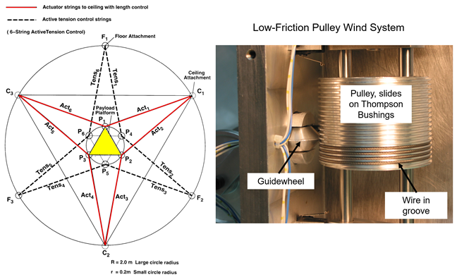
Figure 14: Left: Hexastring arrangement for supporting platform, right: pully wind system
Instead, a platform was built, suspended from six position-controlled servo pulleys at the ceiling and six tension-controlled pulleys at the floor, as shown in the plan view diagram of Figure 14 left. The ceiling wires are depicted in red. One of these pulleys is shown in Figure 14 right, and shows the grooves in the pulley about which the wire is wound. This hexastring configuration is identical to an inverted Steward six-degrees-of-freedom motion platform. The operating volume of the platform was about two meters square and three meters high. The platform could move at a speed of 1 meter per second. The actual instrumented platform was mounted on a 7th degree of freedom that allowed all-attitude yaw about the vertical axis. A camera, three-axis rate gyro and three-axis accelerometer was mounted on this platform which is shown in Figure 15.
In contrast to the upright Steward platform which uses ridged linear actuators, the inverted hexastring configuration has the limitation that the wires can only take tension in one direction. If the platform would move in a position in which one of the wired would become slack, the system would no longer be statically defined. Therefore, the six additional tension-controlled pulleys were placed on the floor. A complex algorithm was developed to compute the tension needed in each one of the wires to prevent the supporting strings from becoming slack. Although the tension control system worked well and increased the operating volume of the platform, it was used very little, since the wires from the floor limited access to the platform and impaired the general mobility in the room.
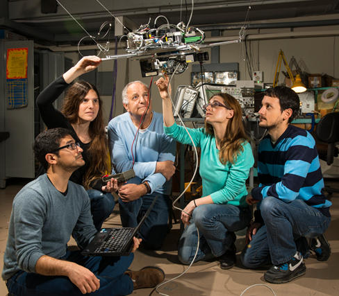
Figure 15: Hovering vehicle simulator platform, suspended by six length-controlled wires
Concluding remarks
The numerous hardware developments described in detail during the existence of the laboratory, demonstrate the need for creative thinking, when no other options are available or out of reach of your budget. This is especially true today, although the focus has shifted from creating hardware to the creative synthesis of existing commercially available hardware and software components. Similar to visual flight simulation, which has shifted from servo-controlled mirrors and cameras to complex computer-generated imagery, hardware has shifted to intelligent software solutions. An example is the quadcopter, where control has moved from mechanically complex servo-controlled swash plates to software-driven speed-controlled rotors. Heavy and expensive gyros and accelerometers are replaced by a single, small, solid-state chip, which also includes a magnetometer and GPS receiver. Accuracy is achieved by complex Kalman Filtering algorithms for blending the sensor data. It is hard to imagine that the Data General Nova 2 computer was once considered a leap in our abilities, in view of today’s low-cost and readily available computational devices, like embedded processors, the Arduino, the Pixhawk or the Raspberry Pie.
Today there is no longer the need to invent the wheel because anything you can think of, has already been done in one form or another. Design tools like Solidworks, linked to 3-D printing, facilitate fast prototyping of mechanical parts, that earlier would take months to develop and manufacture. It would take a long process through the drawing room and mechanical workshop. However, in order to effectively work with these tools, it would be greatly advantageous to have a basic understanding of stereometry, being able to make sketches by hand, having once worked on a lathe and understanding manufacturing methods and materials. Matlab evolved from a linear algebra package to a sophisticated research and design tool, covering a wide range of disciplines. However, in order to effectively use Matlab’s toolboxes, one needs to have a basic understanding of control theory, neural nets, fuzzy logic, signal processing, etc. Object oriented languages like C++ have eliminated the need for developing programs from scratch. Software development now involves the synthesis of ready components and programs. An example is the Unity graphics programming environment used in the gaming community. In order to create a realistic visual urban traffic scene, it is no longer necessary to create a car, a tree, a house or a traffic sign. These objects are readily available on the internet. However, in order to effectively use the program, one needs to understand the basics of viewpoint transformations, projections, three-dimensional rendering, surface texture, lighting, etc.
Lately, flight control evolved from automatic to autonomous AI systems. The technology for these self-learning systems is now available. The advent of affordable 3-D sensor technology like LiDAR and electro-optical sensors paired with fast processors made simultaneous localization and modelling of the environment possible in real time. The emphasis is now on software development and synthesizing existing plug-and-play hardware components. It is clear that, like the Data General Eclipse computer, now displayed in the Madatech museum, also today’s top of the line hardware and software techniques will rapidly evolve into newer equipment and ideas, and new horizons will open up.
– Written by Prof. (ret.) Arthur Grunwald